What Is a PID Controller?

A PID controller is an industrial automation control system that continually adjusts an output to keep a process variable - such as speed, temperature, pressure, or level - at (or as near as possible to) a desired target known as the setpoint.

PID Controllers work by measuring the difference between what you want (the setpoint) and what’s actually happening (the process variable). This difference is called the error. The controller then calculates how much correction is needed and adjusts its output to reduce that error.

For example, in a heating system, if the temperature drops below the setpoint, the PID controller increases power to the heater until the temperature rises back to where it should be.

What Does “PID” Stand For?

PID stands for Proportional, Integral, and Derivative - the three mathematical functions the controller uses to decide how much correction to apply.

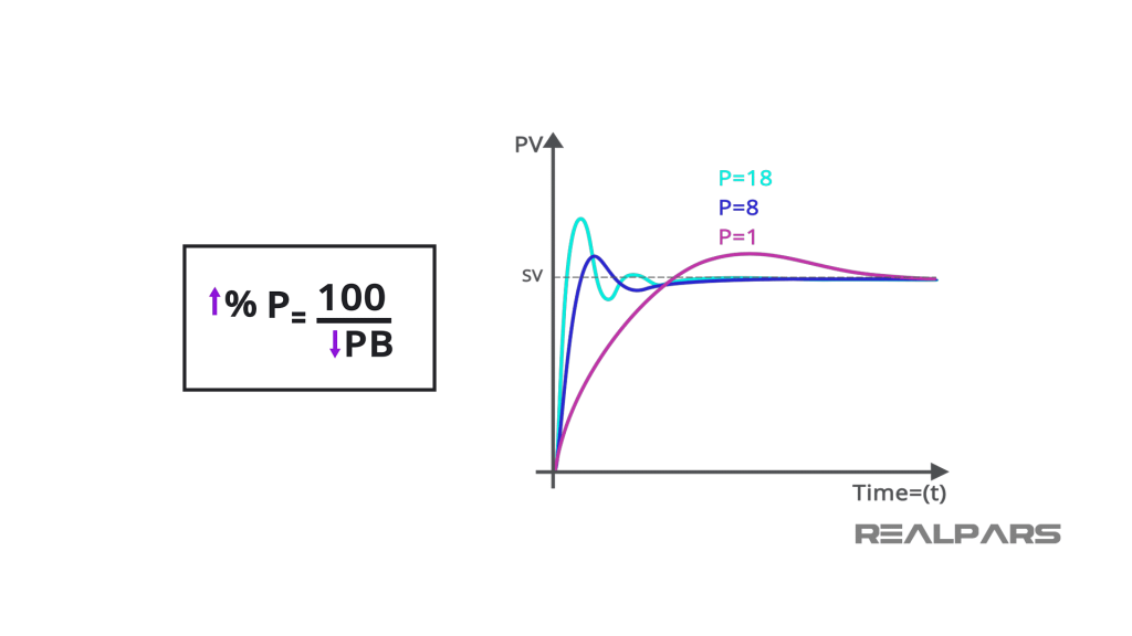
Proportional (P)

The proportional term responds to the current error. If the process is far from the setpoint, the controller makes a large correction. As it gets closer, the correction becomes smaller. This helps the system react quickly but can leave a small steady error or cause overshoot if set too aggressively.

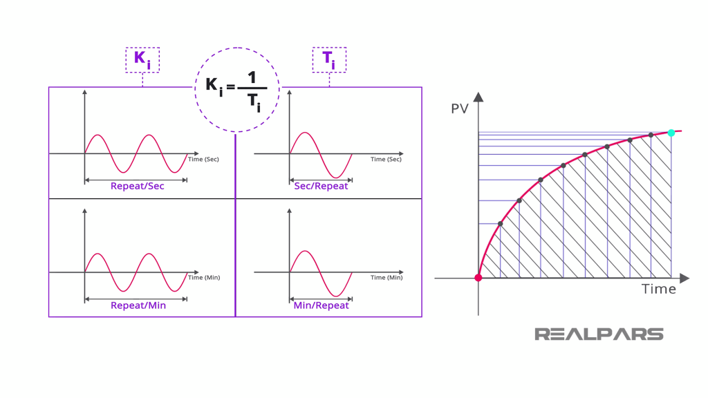
Integral (I)

The integral term looks at the accumulated error over time. If the process has been sitting slightly below the setpoint for a while, the integral term builds up and pushes the output higher until the steady error is gone. This ensures the system settles exactly at the setpoint, but too much integral action can make it sluggish or unstable.

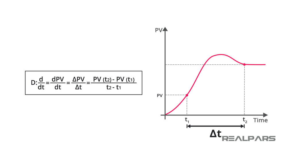
Derivative (D)

The derivative term predicts future error by measuring how quickly the process variable is changing.
It acts as a damping force, helping to prevent overshoot and oscillation. This makes the system smoother and more stable, though it can be sensitive to noisy signals.

The combination of these three effects means your controller can respond quickly, eliminate long-term error, and remain stable - keeping your industrial processes running smoothly.

The PID Equation

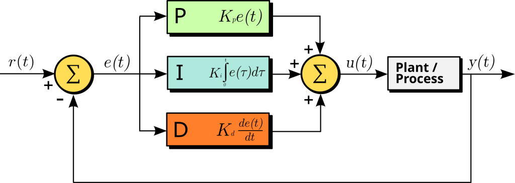
At the heart of every PID controller is the PID equation. This is the mathematical model that uses the Proportional, Integral and Derivative data to determine what correction to make. The general form looks like this:

Output = (Kp × Error) + (Ki × Integral of Error) + (Kd × Derivative of Error)

So in a PID equation, the p, i, and d each indicate a part of the control action, while the K stands for a gain constant - a fixed multiplier that determines how strongly that part of the controller reacts.

Why "k"? A Little Historical Context

The PID controller’s roots go back to the early 1900s, when proportional–integral control was first used in steam engine governors. When the derivative component was added in the 1930s, the full “PID” structure emerged.

The letter K is traditionally used in engineering and physics to represent a constant of proportionality - a number that scales or adjusts the effect of something. By the time modern electronic and pneumatic controllers were being designed in the mid-20th century, the Kp, Ki, Kd notation had already become standard through academic control theory papers and military engineering specifications.

Measuring the Error

So, the PID controller constantly measures the process variable (for example, motor speed or temperature) using a sensor such as a thermocouple, pressure transducer or encoder. It compares this reading to the setpoint, which is the target value entered by the user. The difference between the two is the error:

Error = Setpoint − Process Variable

If the process is below the setpoint, the error is positive and the controller increases its output accordingly. If it’s above, the error is negative and the controller decreases the output.

The Proportional Term (Kp × Error)

This part gives an output directly proportional to the size of the error. It is the controller’s immediate reaction. If the error doubles, the proportional term doubles too. A high Kp gain makes the system respond more quickly, but can also cause overshoot and oscillation if set too high. In a real controller, this term is recalculated many times per second, producing a rapid feedback response that tracks the current difference between setpoint and measurement.

The Integral Term (Ki × Integral of Error)

The integral term looks at error accumulated over time. Each cycle, the controller adds up the small errors that have built up and multiplies that total by Ki. If the process has been slightly below the setpoint for a long time, the integral value keeps growing until the controller output increases enough to remove the persistent offset.

In electronic form, this “integral” is usually implemented by summing a series of past error samples rather than performing continuous integration. Many digital controllers also include a limit (often called an anti-wind-up function) to prevent the integral term from growing too large when the output is already at its maximum.

The Derivative Term (Kd × Derivative of Error)

The derivative term estimates the rate of change of the error. It predicts how the error is moving - whether it’s increasing or decreasing - and reacts before the process overshoots. Mathematically, it is the slope of the error curve. If the error is changing quickly, the derivative term produces a larger corrective signal that slows the response.

In a digital PID, this derivative is found by comparing the current error with the previous one and dividing by the time between updates. Because it responds strongly to rapid fluctuations, some controllers apply filtering to smooth out noise in the measurement signal.

How the Equation Is Executed in Practice

Modern PID controllers run this calculation automatically inside a control loop that repeats at regular intervals - often every few milliseconds. Each loop follows the same cycle:

1. Measure the process variable through a sensor input.
2. Calculate the error between setpoint and measurement.
3. Compute each term of the PID equation (proportional, integral and derivative).
4. Sum the three results to determine the new output value.
5. Send the output to an actuator, such as a motor, valve or heater.
6. Repeat continuously to maintain control as conditions change.

This constant feedback loop allows the controller to adjust in real time. Even if the system is disturbed - by a change in load, supply voltage or ambient conditions, for example - the PID controller recalculates almost instantly and corrects the output.

Understanding the Effect of Each Term

You can think of the three components as working together like a team:

• P acts like a strong, quick correction based on the present.
• I provides patience and persistence, gradually removing any lingering offset.
• D offers foresight, damping sudden movements before they cause instability.

Tuning the constants Kp, Ki and Kd changes how the team behaves. Some applications benefit from a fast, assertive response (large Kp, small Ki), while others need gentler control with strong damping (smaller Kp, more Kd).

Tuning a PID Controller

To work effectively, each system needs its PID parameters tuned correctly. This means adjusting the three constants (Kp, Ki, and Kd) so that the process responds quickly but without overshoot or oscillation.
Here are some practical tips:

• Start by increasing Kp until you achieve a fast, stable response.
• Add a small Ki to eliminate steady-state error.
• Introduce Kd to smooth the reaction and prevent overshoot.
  Many modern digital controllers include auto-tuning functions (often available with products like those above) that calculate optimal settings automatically, making setup faster and easier.

Digital Implementation

In most modern equipment, PID control is handled by a microprocessor or PLC running a digital algorithm. The continuous equation is translated into a discrete form that updates at each sample time Δt:

Output[n] = Output[n−1] + Kp × (Error[n] − Error[n−1]) + Ki × Error[n] × Δt + Kd × (Error[n] − 2×Error[n−1] + Error[n−2]) / Δt

This digital method lets the controller run on standard PLC hardware, ensuring consistent results while allowing easy adjustment of the gains and timing.

Why This Matters

Understanding how the PID equation works helps engineers fine-tune systems more effectively. It explains why increasing Kp makes the response quicker, why too much Ki causes overshoot, and how Kd can stabilise an otherwise restless process. So your PID Controller is measuring, comparing, and correcting your process continuously for stable, precise automation.

Where Are PID Controllers Used?

PID controllers are found in almost every corner of industrial automation, because so many processes involve maintaining a constant condition, whether that’s speed, pressure, flow, or temperature. Any time you need a system to stay steady in the face of change, there’s a good chance a PID loop is working behind the scenes. For instance:

Temperature and Process Control

One of the most common uses of PID control is in temperature regulation. Heating and cooling systems rely on PID loops to hold a setpoint without overshoot. Using PID logic to keep temperatures stable in furnaces, ovens, or environmental chambers.

These standalone controllers constantly measure the temperature through a sensor (such as a thermocouple or RTD), compare it with the desired setpoint, and adjust the output to heaters or cooling elements automatically.

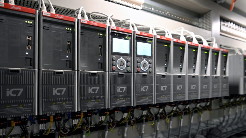
Motor Speed and Torque Regulation

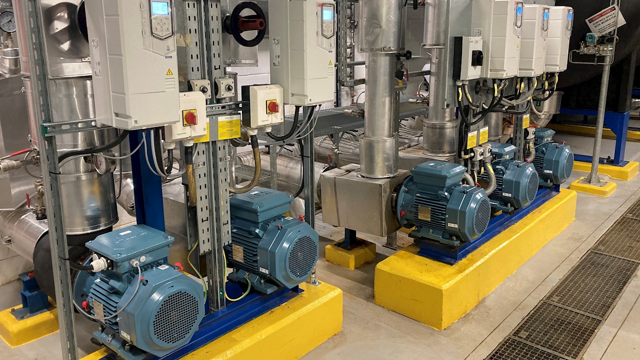
PID control is also built directly into many variable speed drives (VSDs) or inverters. These loops allow the drive to maintain a constant motor speed, flow rate, or pressure automatically, even if the load or system resistance changes. In pump or fan VSD applications, this means the drive can intuitively increase or reduce motor speed to keep the process stable, saving energy while protecting the equipment.

Pressure and Flow Control

In pumping systems, maintaining consistent pressure or flow is critical. Rather than running motors at a fixed speed, a PID-controlled drive monitors feedback from a pressure or flow sensor and adjusts output dynamically. Products like the Danfoss VLT range are designed specifically for this kind of work, offering dual PID loops to handle complex multi-pump arrangements or fan arrays.

Level Control in Tanks and Vessels

In process industries, liquid levels must often stay within tight limits. A PID controller can balance inflow and outflow by adjusting valves or pumps based on level sensor feedback. This type of application often uses compact PLC systems such as the Unitronics Vision series, which combine logic control, PID loops, and a touch-screen HMI in a single integrated unit.

Motion Control and Robotics

In robotics and CNC systems, PID loops control motor position and speed with extreme precision. Even tiny deviations are corrected almost instantly, ensuring accurate motion and repeatability.
You’ll often see this in servo drive applications, many of which are compatible with the automation platforms and control accessories supplied by LED Controls.

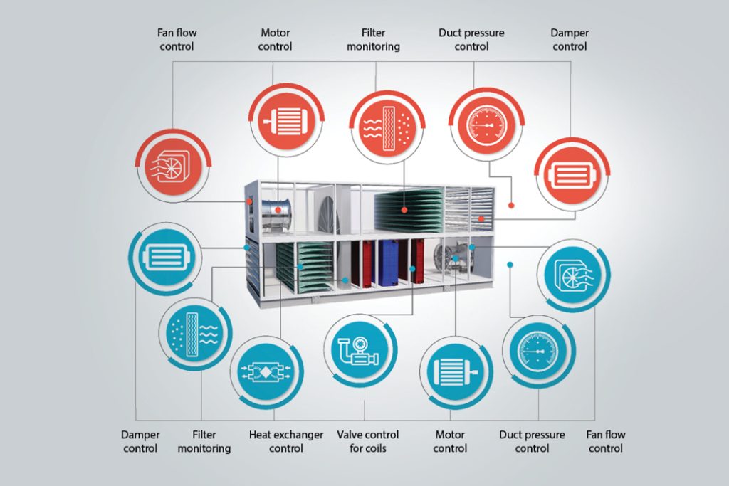
Environmental and HVAC Systems

PID control is also used in heating, ventilation and air-conditioning (HVAC) systems to regulate temperature, humidity and airflow efficiently.

In each case, the PID controller provides the same essential service - continuously monitoring a process, calculating the difference from the target, and making fine-tuned adjustments to achieve stable, reliable operation.

Recommended PID-Capable Products from LED Controls

Manufacturer	Model / Type	Key PID / Control Features	Why Consider It
Danfoss	Danfoss VLT series Drives	These drives offer process-control features (e.g. PI/PID loops) built-in for pumps, fans, HVAC and general automation	Great for variable speed drives with process-control capability (e.g. flow, pressure)
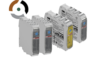
ABB	VSD range	VFDs from ABB include built-in control loops and advanced algorithms	Ideal where you need motor speed or torque control and want a PID loop integrated in the drive.
IMO	IMO Jaguar VXR Variable Speed Drive	“PID with Dancer control” and multiple PID loops as features.	Good choice for high-performance VSDs with built-in PID loops for pumps, conveyors etc.
Unitronics	Unitronics Vision / PLC + HMI Controllers	This all-in-one PLC + HMI platform supports PID function blocks and integrated control logic.	Best when you want full programmable logic + PID loops in one device (not just motor drives)

At LED Controls, our team can help you select the right PID equipment, ensure correct loop configuration for your process and get your system operating with maximum efficiency and reliability. Get in touch to find out more.